Two-body fix (Santa Barbara, 16 July 2011)

A recent trip to Santa Barbara, California, presented me with an opportunity to do some sights and calculations. In the following example I took a series of Sun sights in the morning and a single sight in the afternoon.  The four morning sights were averaged to produce a single effective data point, whose LOP was then crossed with the LOP from the afternoon sight to obtain a fix.

Observation point:
Google Earth coordinates: Santa Barbara Sailing Club beach
N    34º 24.18′    i.e.    34.403
º
W 119º 41.64′    i.e. -119.694
º

These coordinates were used as the “assumed position” (AP) in the subsequent calculations of intercepts and azimuths.

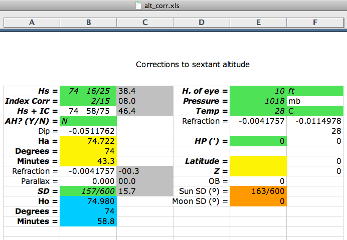
Sun semidiameter (SD) = 15.7′

Sextant: Davis Mark 15

16 July 2011 (Sun: morning):  T=25 ºC,  P=1011 mb,  Index Correction=+8.0′,  Height of eye=6 ft
UT               Hs               Ho               GHA            Declination   Intercept    Azimuth
17:42:30      55° 48.2′     56° 08.9′      84° 06.4′      N 21° 19.9′       0.4A         103.3
17:45:20      56° 23.4′     56° 44.1′      84° 48.9′      N 21° 19.8′       0.8T         103.9
17:47:50      56° 51.6′     57° 12.3′      85° 26.4′      N 21° 19.8′       1.0A         104.4
17:50:30      57° 22.4′     57° 43.1′      86° 06.4′      N 21° 19.8′       2.1A         105.0

The spreadsheet average2.xls results in a simple average of these four observed altitudes:

average2.xls:

that is:
UT               Hs               Ho               GHA            Declination   Intercept    Azimuth
17:46:32       —               56° 57.1′      85° 06.9′      N 21° 19.8′       0.6A         104.1

The single afternoon sight was (this time the sextant’s mirrors were adjusted to eliminate index error):
16 July 2011 (Sun: afternoon):  T=26 ºC,  P=1010 mb,  Index Correction=0.0′,  Height of eye=6 ft
UT               Hs               Ho               GHA            Declination   Intercept    Azimuth
21:18:20      69° 00.6′     69° 13.6′     138° 03.7′     N 21° 18.4′       1.6T          235.8

The two LOP intersections can be computed either with spreadsheet lops.xls or two_body_fix.xls.

two_body_fix.xls:

Solution #1 is relevant in our case:

N    34º 22.8′
W 119º 42.8′

This fix is only 1.7 nm bearing 215 from the Google Earth coordinates, as seen both from:

sailings.xls:

and a Google Earth measurement:

Overall I think I can be reasonably happy with these results and the intercepts I got. Considering the difficulties I had with the index error determination I was in fact a bit worried before I started the calculations. The error of fix and the standard deviation of intercepts are interestingly similar at about 2 nm. Using this value as the “Scatter” parameter in the weighted least-squares fitting procedure (average2.xls: fitted, not precomputed slope), all weights came out equal, so this procedure resulted in calculating the simple average of UT’s and Ho’s.

(first published on September 1, 2011)

Noon curve: Santa Barbara (17 July 2011)

A recent trip to Santa Barbara, California, presented me with an opportunity to do some sights and calculations. In the following example I took a series of Sun sights not long before the Local Apparent Noon (LAN). I was unable to stay long enough to observe the actual meridian upper transit of the Sun but the data were still suitable for a noon-curve construction by extrapolation and thus establishing the latitude and longitude of my location with decent enough accuracy.

Observation point:
Google Earth coordinates: Santa Barbara Sailing Club beach
N    34º 24.18′    i.e.    34.403
º
W 119º 41.64′    i.e. -119.694
º

These coordinates were used as the “assumed position” (AP) in the subsequent calculations of intercepts and azimuths.

Sun semidiameter (SD) = 15.7′

Sextant: Davis Mark 15

17 July 2011 (Sun: just before LAN):  T=28 ºC,  P=1018 mb,  Index Correction=+8.0′,  Height of eye=10 ft
UT             Hs              Ho             GHA            Declination   Intercept    Azimuth
19:33:30    74º 38.4′    74º 58.8′    111º 50.0′     N 21º 09.0′     4.0A           150.4
19:35:30    74º 55.4     75º 15.8′    112º 20.0′     N 21º 09.0′    1.1T            152.0
19:37:55    75º 09.4′    75º 29.8′    112º 56.2′     N 21º 09.0′    1.5T            154.1
19:40:30    75º 16.2′    75º 36.6′    113º 35.0′     N 21º 09.0′    5.1A            156.3
19:43:00    75º 34.0′    75º 54.4′    114º 12.5′     N 21º 08.9′    0.9T            158.5
19:46:00    75º 45.0′    76º 05.4′    114º 57.5′     N 21º 08.9′    0.8A            161.3
19:49:50    75º 58.6′    76º 19.0′    115º 55.0′     N 21º 08.9′    1.0A            164.9
19:53:30    76º 08.0′    76º 28.4′    116º 50.0′     N 21º 08.9′    2.1A            168.5
19:57:30    76º 14.8′    76º 35.2′    117º 50.0′     N 21º 08.8′    3.4A            172.5

Observed altitudes (Ho) were obtained from the recorded sextant altitudes (Hs) with alt_corr.xls; see the first data point as an example (these were lower-limb observations, hence the SD correction is positive).

alt_corr.xls

The Sun GHA, Declination, SD, and (later) Equation-of-Time values came from sun.xls. The intercept and azimuth were calculated with intercept.xls. The intercept distances are small as expected, since they were calculated using the known position as the AP. The fact that the intercepts are not exactly zero is a measure of the quality of the instrument and the skill of the person using it. The azimuths approach the meridian passage value of 180º but stop just short of it due to reasons explained above.

In the following image we can indeed see a rather convincing arc that would peak shortly after 20^h UT. This plot has the Ho’s on the y-axis.

Before the actual fitting these Ho’s are further adjusted to account for the Sun’s hourly declination change of -0.4′. In addition, the noon_motion.xls spreadsheet is also capable of addressing the construction of this curve on a moving vessel; in this case the speed is zero since I made the observations from a fixed location.

noon_motion.xls

The results are computed by noon_motion.xls to be:

N    34º 29.1′
W 119º 24.5′

One generally expects getting a very accurate latitude value and not-so-great longitude value from meridian-transit observations. In the past I have observed that the parabolic fitting employed by these spreadsheets works very well if the data actually straddle the culmination point. This computed result is not as good but it is still reasonable, especially since it came from a data set that stopped short of LAN and hence had to be extrapolated.

(first published on July 31, 2011)